
17 what form an analog signal can have. How is a measurement signal different from a signal? Give examples of measuring signals used in various branches of science and technology
How is a measurement signal different from a signal? Give examples of measuring signals used in various branches of science and technology
The measuring signal is a material carrier of information containing quantitative information about the measured physical quantity and representing a certain physical process, one of the parameters of which is functionally related to the measured physical quantity. This parameter is called informative. And the signal carries quantitative information only about the informative parameter, and not about the measured physical quantity.
Examples of measurement signals can be
Output signals of various generators (magnetohydrodynamic, lasers, masers, etc.), transformers (differential, current, voltage)
Various electromagnetic waves (radio waves, optical radiation, etc.)
List the features by which measuring signals are classified
By the nature of the measurement of informative and temporal parameters, the measuring signals are divided into analog, discrete and digital. According to the nature of the change in time, the signals are divided into constant and variable. According to the degree of availability of a priori information, variable measuring signals are divided into deterministic, quasi-deterministic and random.
What is the difference between analog, discrete and digital signals?
An analog signal is a signal described by a continuous or piecewise continuous function Y a (t), and both this function itself and its argument t can take any values on the given intervals (Y min ; Y max) and (t min ; t max).
A discrete signal is a signal that changes discretely in time or in level. In the first case, it can receive at discrete times nT, where T = const is the sampling interval (period), n = 0; one; 2; ... - an integer, any values in the interval (Y min ; Y max) called samples, or readings. Such signals are described by lattice functions. In the second case, the values of the signal Yd(t) exist at any time t in the interval (t min ; t max), however, they can take a limited number of values h j = nq, multiples of the q quantum.
Digital signals - signals quantized in level and discrete in time signals Y q (nT), which are described by quantized lattice functions (quantized sequences) that at discrete times nT take only a finite series of discrete values - quantization levels h 1 h 2 , ... , h n .
Tell us about the characteristics and parameters of random signals
A random signal is a time-varying physical quantity, whose instantaneous value is a random variable.
The family of realizations of a random process is the main experimental material on the basis of which its characteristics and parameters can be obtained.
Each implementation is a non-random function of time. The family of realizations for any fixed value of time t o is a random variable, called the section of the random function corresponding to the time t o . Therefore, the random function combines characteristics random variable and deterministic function. With a fixed value of the argument, it turns into a random variable, and as a result of each individual experiment, it becomes a deterministic function.
The most complete random processes are described by distribution laws: one-dimensional, two-dimensional, etc. However, it is very difficult to operate with such, in the general case, multidimensional functions, therefore, in engineering applications, such as metrology, they try to get by with the characteristics and parameters of these laws, which describe random processes not completely, but partially. Characteristics of random processes, in contrast to the characteristics random variables, which are discussed in detail in Chap. 6 are not numbers, but functions. The most important of them are the mathematical expectation and variance.
The mathematical expectation of a random function X(t) is a non-random function
mx(t) = M = xp(x, t)dx,
which for each value of the argument t is equal to the expectation of the corresponding section. Here p(x, t) is the one-dimensional distribution density of the random variable x in the corresponding section of the random process X(t). Thus, the mathematical expectation in this case is an average function around which specific implementations are grouped.
The variance of a random function X(t) is a non-random function
Dx(t) = D = 2p(x, t)dx,
the value of which for each moment of time is equal to the variance of the corresponding section, i.e. the variance characterizes the spread of realizations with respect to mx(t).
The mathematical expectation of a random process and its variance are very important, but not exhaustive, characteristics, since they are determined only by a one-dimensional distribution law. They cannot characterize the relationship between different sections of a random process when different values time t and t". For this, a correlation function is used - a non-random function R(t, t") of two arguments t and t", which, for each pair of values of the arguments, is equal to the covariance of the corresponding sections of the random process:
A correlation function, sometimes called an autocorrelation function, describes the statistical relationship between the instantaneous values of a random function separated by set value time φ \u003d t "-t. If the arguments are equal, the correlation function is equal to the variance of the random process. It is always non-negative.
In practice, the normalized correlation function is often used
It has the following properties: 1) if the arguments t and t are equal, r(t, t") = 1; 2) is symmetrical with respect to its arguments: r(t,t") = r(t",t); 3) its possible values lie in the range [-1;1], i.e. |r(t,t")| ? 1. The normalized correlation function is similar in meaning to the correlation coefficient between random variables, but depends on two arguments and is not a constant value.
Random processes that proceed uniformly in time, particular implementations of which oscillate around the average function with a constant amplitude, are called stationary. :Quantitatively, the properties of stationary processes are characterized by the following conditions.
* Mathematical expectation of a stationary process is constant, I.e. m x (t) = m x = const. However, this requirement is not essential, since it is always possible to pass from a random function X(t) to a centered function, for which the mathematical expectation is zero. It follows from this that if a random process is non-stationary only due to the variable in time (along the sections) mathematical expectation, then by the operation of centering it can always be reduced to a stationary one.
* For a stationary random process, the variance over sections is a constant value, i.e. Dx(t) = Dx = const.
* : The correlation function of a stationary process does not depend on the value of the arguments t and t ", but only on the interval φ = t" -t, i.e. R(t,t") = R(f). The previous condition is a special case of this condition, i.e. Dx(t) = R(t, t) = R(f = O) = const. Thus, the dependence autocorrelation function only from the interval "t is the only essential condition stationarity of a random process.
An important characteristic of a stationary random process is its spectral density S(w), which describes the frequency composition of the random process at w?0 and expresses the average power of the random process per unit frequency band:
The spectral density of a stationary random process is a non-negative function of the frequency S(w)?0. The area under the S(w) curve is proportional to the dispersion of the process. The correlation function can be expressed in terms of the spectral density
R (f) \u003d S (u) cosshfdsh.
Stationary random processes may or may not have the ergodicity property. A stationary random process is called ergodic if any of its realizations of sufficient duration is, as it were, an "authorized representative" of the entire set of process realizations. In such processes, any implementation will sooner or later go through any state, regardless of what state this process was in at the initial moment of time.
Probability theory and mathematical statistics are used to describe the errors. However, a number of important caveats must first be made:
* application methods mathematical statistics to the processing of measurement results is competent only on the assumption that the individual received readings are independent of each other;
* most of the formulas of probability theory used in metrology are valid only for continuous distributions, while the distributions of errors due to the inevitable quantization of readings, strictly speaking, are always discrete, i.e. error can only be countable set values.
Thus, the conditions of continuity and independence for the measurement results and their errors are observed approximately, and sometimes they are not observed. In mathematics, the term "continuous random variable" means a much narrower concept, limited by a number of conditions, than "random error" in metrology.
Given these limitations, the process of the appearance of random errors in the results of measurements, minus systematic and progressive errors, can usually be considered as a centered stationary random process. Its description is possible on the basis of the theory of statistically independent random variables and stationary random processes.
When performing measurements, it is required to quantify the error. For such an assessment, it is necessary to know certain characteristics and parameters of the error model. Their nomenclature depends on the type of model and the requirements for the estimated error. In metrology, it is customary to distinguish three groups of characteristics and error parameters. The first group - given as the required or allowable norms of measurement error characteristics (error standards). The second group of characteristics is the errors attributed to the totality of measurements performed according to a certain methodology. The characteristics of these two groups are used mainly for mass technical measurements and represent the probabilistic characteristics of the measurement error. The third group of characteristics - statistical estimates of measurement errors reflect the proximity of a separate, experimentally obtained measurement result to the true value of the measured quantity. They are used in the case of measurements carried out in scientific research and metrological work.
RMS of the random component of the measurement error and, if necessary, its normalized autocorrelation function are used as characteristics of the random error.
The systematic component of the measurement error is characterized by:
* RMS of the non-excluded systematic component of the measurement error;
* the boundaries within which the non-excluded systematic component of the measurement error is located with a given probability (in particular, with a probability equal to one).
Requirements for accuracy characteristics and recommendations for their selection are given in normative document MI 1317-86 "GSI. Results and characteristics of measurement errors. Forms of presentation. Methods of use in testing product samples and monitoring their parameters."
A signal is defined as a voltage or current that can be transmitted as a message or as information. By their nature, all signals are analog, whether DC or AC, digital or pulsed. However, it is customary to make a distinction between analog and digital signals.
A digital signal is a signal that has been processed in a certain way and converted into numbers. Usually these digital signals are connected to real analog signals, but sometimes there is no connection between them. An example is the transmission of data in local area networks (LANs) or other high-speed networks.
In the case of digital signal processing (DSP), an analog signal is converted into binary form by a device called an analog-to-digital converter (ADC). The output of the ADC is a binary representation of the analog signal, which is then processed by an arithmetic digital signal processor (DSP). After processing, the information contained in the signal can be converted back to analog form using a digital-to-analog converter (DAC).
Another key concept in defining a signal is the fact that a signal always carries some information. This brings us to the key problem of processing physical analog signals - the problem of information extraction.
Purposes of signal processing.
The main purpose of signal processing is the need to obtain the information contained in them. This information is usually present in the amplitude of the signal (absolute or relative), in frequency or spectral content, in phase or in the relative time dependences of several signals.
Once the desired information has been extracted from the signal, it can be used in a variety of ways. In some cases, it is desirable to reformat the information contained in the signal.
In particular, the change in signal format occurs when an audio signal is transmitted in a frequency division multiple access (FDMA) telephone system. In this case, analog methods are used to accommodate multiple voice channels in the frequency spectrum for transmission via microwave radio relay, coaxial or fiber optic cable.
In the case of digital communication, analog audio information is first converted to digital using an ADC. The digital information representing the individual audio channels is time multiplexed (Time Division Multiple Access, TDMA) and transmitted over a serial digital link (as in a PCM system).
Another reason for signal processing is to compress the signal bandwidth (without significant loss of information), followed by formatting and transmission of information at reduced speeds, which can narrow the required channel bandwidth. High-speed modems and adaptive pulse code modulation (ADPCM) systems make extensive use of data de-redundancy (compression) algorithms, as do digital mobile communication systems, MPEG audio recording systems, and high-definition television (HDTV).
Industrial data acquisition and control systems use information received from sensors to generate appropriate feedback signals, which in turn directly control the process. Note that these systems require both ADCs and DACs, as well as sensors, signal conditioners, and DSPs (or microcontrollers).
In some cases, there is noise in the signal containing information, and the main goal is to restore the signal. Techniques such as filtering, autocorrelation, convolution, etc. are often used to accomplish this task in both the analog and digital domains.
PURPOSE OF SIGNAL PROCESSING- Extraction of signal information (amplitude, phase, frequency, spectral components, timing)
- Signal format conversion (telephony with channel division FDMA, TDMA, CDMA)
- Data compression (modems, Cell Phones, HDTV TV, MPEG compression)
- Formation of feedback signals (industrial process control)
- Extraction of signal from noise (filtering, autocorrelation, convolution)
- Extraction and storage of a signal in digital form for further processing (FFT)
Signal conditioning
In most of the above situations (associated with the use of DSP technologies), both an ADC and a DAC are needed. However, in some cases only a DAC is required when analog signals can be directly generated based on DSP and DAC. A good example is video-scan displays, in which a digitally generated signal drives the video image or a RAMDAC (Digital to Analogue Array of Pixel Value Converter) block.
Another example is artificially synthesized music and speech. In fact, when generating physical analog signals using only digital methods, they rely on information previously obtained from sources of similar physical analog signals. In display systems, the data on the display must convey relevant information to the operator. When developing sound systems are given by the statistical properties of the generated sounds, which have been previously determined using extensive DSP methods (sound source, microphone, preamplifier, ADC, etc.).
Signal processing methods and technologies
Signals can be processed using analog techniques (analog signal processing, or ASP), digital techniques (digital signal processing, or DSP), or a combination of analog and digital techniques (combined signal processing, or MSP). In some cases, the choice of methods is clear, in other cases there is no clarity in the choice and the final decision is based on certain considerations.
With regard to DSP, its main difference from traditional computer data analysis lies in the high speed and efficiency of complex digital processing functions, such as filtering, real-time data analysis and compression.
The term "combined signal processing" implies that the system performs both analog and digital processing. Such a system can be implemented as a printed circuit board, a hybrid integrated circuit (IC), or a single chip with integrated elements. ADCs and DACs are considered to be combined signal processing devices, since both analog and digital functions are implemented in each of them.
Recent advances in very high integration (VLSI) chip technology enable complex (digital and analog) processing on a single chip. The very nature of DSP implies that these functions can be performed in real time.
Comparison of analog and digital signal processing
Today's engineer is faced with the choice of the proper combination of analog and digital methods to solve a signal processing problem. It is impossible to process physical analog signals using only digital methods, since all sensors (microphones, thermocouples, piezoelectric crystals, storage heads on magnetic disks etc.) are analog devices.
Some types of signals require the presence of normalization circuits for further processing of signals in both analog and digital methods. Signal conditioning circuits are analog processors that perform functions such as amplification, accumulation (in instrumentation and pre-amplifiers (buffer) amplifiers), signal detection against background noise (by high-precision common-mode amplifiers, equalizers, and linear receivers), dynamic range compression (by logarithmic amplifiers, logarithmic DACs and PGAs) and filtering (passive or active).
Several methods for implementing the signal processing process are shown in Figure 1. The upper area of the figure depicts a purely analog approach. The rest of the areas show the implementation of the DSP. Note that once a DSP technology is chosen, the next decision must be to locate the ADC in the signal processing path.
ANALOG AND DIGITAL SIGNAL PROCESSING
Figure 1. Signal processing methods
In general, since the ADC has been moved closer to the sensor, most of the analog signal processing is now done by the ADC. Increasing the capabilities of the ADC can be expressed in increasing the sampling rate, expanding the dynamic range, increasing the resolution, cutting off the input noise, using input filtering and programmable amplifiers (PGA), the presence of on-chip voltage references, etc. All the add-ons mentioned increase the functional level and simplify the system.
In the presence of modern technologies In the production of DACs and ADCs with high sampling rates and resolutions, significant progress has been made in integrating more and more circuits directly into the ADC/DAC.
In the field of measurement, for example, there are 24-bit ADCs with built-in programmable amplifiers (PGAs) that allow you to digitize full-scale 10 mV bridge signals directly, without subsequent normalization (for example, the AD773x series).
At voice and audio frequencies, complex encoding-decoding devices are common - codecs (Analog Front End, AFE), which have an analog circuit built into the chip that meets the minimum requirements for external normalization components (AD1819B and AD73322).
There are also video codecs (AFE) for applications such as CCD image processing (CCD) and others (such as the AD9814, AD9816, and AD984X series).
Implementation example
As an example of using DSP, let's compare analog and digital low-pass filters (LPF), each with a cutoff frequency of 1 kHz.
The digital filter is implemented as the typical digital system shown in Figure 2. Note that the diagram makes several implicit assumptions. First, to accurately process the signal, it is assumed that the ADC/DAC path has sufficient sample rate, resolution, and dynamic range. Secondly, in order to complete all of its calculations within the sampling interval (1/f s), the DSP device must be fast enough. Thirdly, at the input of the ADC and the output of the DAC, there is still a need for analog filters for limiting and restoring the signal spectrum (anti-aliasing filter and anti-imaging filter), although the requirements for their performance are low. With these assumptions in mind, the digital and analog filters can be compared.

Figure 2. Block diagram of a digital filter
The required cutoff frequency for both filters is 1 kHz. The analog conversion is implemented by a sixth-order Chebyshev filter of the first kind (characterized by the presence of gain ripple in the passband and the absence of ripple outside the passband). Its characteristics are shown in Figure 2. In practice, this filter can be represented by three second-order filters, each of which is built on an operational amplifier and several capacitors. By using modern systems computer-aided design (CAD) filters to create a sixth-order filter is quite simple, but to satisfy technical requirements according to the uneven characteristics of 0.5 dB, an accurate selection of components is required.
The 129-coefficient digital FIR filter shown in Figure 2 has a ripple of only 0.002 dB in the passband, a linear phase response, and a much steeper rolloff. In practice, such characteristics cannot be realized using analog methods. Another obvious advantage of the circuit is that the digital filter does not require component selection and is not subject to parameter drift, since the filter's clock frequency is stabilized by a quartz resonator. A filter with 129 coefficients requires 129 multiply-accumulate (MAC) operations to calculate the output sample. These calculations must be completed within the 1/fs sampling interval to ensure real-time operation. In this example, the sample rate is 10 kHz, so 100 µs is sufficient for processing if no significant additional calculations are required. The ADSP-21xx family of DSPs can complete the entire multiplication-accumulate process (and other functions required to implement a filter) in a single instruction cycle. Therefore, a filter with 129 coefficients requires a speed of more than 129/100 µs = 1.3 million operations per second (MIPS). Existing DSPs are much faster and thus are not a limiting factor for these applications. The 16-bit ADSP-218x fixed-point series achieves up to 75MIPS performance. Listing 1 shows the assembler code that implements the filter on DSP processors of the ADSP-21xx family. Note that the actual lines of executable code are marked with arrows; the rest are comments.

Figure 3. Analog and digital filters
Of course, in practice, there are many other factors that are considered when comparing analog and digital filters or analog and digital signal processing methods in general. Modern signal processing systems combine analog and digital methods to achieve a desired function and take advantage of the best methods, both analog and digital.
ASSEMBLY PROGRAM:
FIR FILTER FOR ADSP-21XX (SINGLE PRECISION)
MODULE fir_sub; ( Filter FIR subroutine Subroutine call parameters I0 --> Oldest data in delay line I4 --> Start of filter coefficient table L0 = Filter length (N) L4 = Filter length (N) M1,M5 = 1 CNTR = Filter length - 1 (N-1) Return values MR1 = Result of summation (rounded and limited) I0 --> Oldest data in delay line I4 --> Start of filter coefficient table Change registers MX0,MY0,MR Running time (N - 1) + 6 cycles = N + 5 cycles All coefficients are in the format 1.15 ) .ENTRY fir; fir: MR=0, MX0=DM(I0,M1), MY0=PM(I4,M5) CNTR=N-1; DO convolution UNTIL CE; convolution: MR=MR+MX0*MY0(SS), MX0=DM(I0,M1), MY0=PM(I4,M5); MR=MR+MX0*MY0(RND); IF MV SAT MR; RTS; .ENDMOD; REAL TIME SIGNAL PROCESSING
Literature:
Together with the article "Types of signals" they read:
The following types of signals are distinguished, which correspond to certain forms of their mathematical description.
Rice. 1.2.1. analog signal.
analog signal (analog signal) is a continuous function of a continuous argument, i.e. defined for any argument value. The sources of analog signals, as a rule, are physical processes and phenomena that are continuous in the dynamics of their development in time, in space or in any other independent variable, while the recorded signal is similar (“similar”) to the process that generates it. An example of mathematical notation of a signal: y(t)= 4.8 exp[-(t-4) 2 /2.8]. An example of a graphical display of this signal is shown in fig. 1.2.1, while both the function itself and its arguments can take any values within certain intervals y 1 y y 2 , t 1 t t 2 . If the intervals of the values of the signal or its independent variables are not limited, then by default they are taken equal to - to +. The set of possible signal values forms a continuum - a continuous space in which any signal point can be determined up to infinity. Examples of signals that are analog in nature are the change in the strength of the electric, magnetic, electromagnetic fields in time and space.

Rice. 1.2.2. discrete signal
discrete signal (discrete signal) in its values is also a continuous function, but defined only in discrete values of the argument. According to the set of its values, it is finite (countable) and is described by a discrete sequence of samples (samples) y(nt), where y 1 y y 2 , t is the interval between samples (interval or sampling step, sample time) , n = 0,1,2,...,N. The reciprocal of the sampling step: f = 1/t is called the sampling frequency. If a discrete signal is obtained by sampling (sampling) an analog signal, then it is a sequence of samples, the values of which are exactly equal to the values of the original signal in terms of nt.An example of sampling an analog signal shown in fig. 1.2.1 is shown in fig. 1.2.2. When t = const (uniform data sampling), the discrete signal can be described by the abbreviation y(n). In the technical literature, in the notation of discretized functions, the former indices of the arguments of analog functions are sometimes left, enclosing the latter in square brackets - y[t]. In case of non-uniform signal sampling, the designations of discrete sequences (in text descriptions) are usually enclosed in curly brackets - (s(t i)), and the values of the samples are given in the form of tables indicating the values of the coordinates t i . For numerical sequences (uniform and non-uniform), the following numerical description is also used: s(t i) = (a 1 ,a 2 , ..., a N ), t = t 1 ,t 2 , ...,t N . Examples of discrete geophysical signals are the results of vertical electrical sounding, geochemical sampling profiles, etc.

Rice. 1.2.3. digital signal
digital signal (digital signal) is quantized in its values and discrete in its argument. It is described by a quantized lattice function y n = Q k , where Q k is the quantization function with the number of quantization levels k, while the quantization intervals can be both uniformly distributed and non-uniformly, for example, logarithmic. A digital signal is specified, as a rule, in the form of a discrete series of numerical data - a numerical array of consecutive values of the argument with t = const, but in the general case, the signal can also be specified in the form of a table for arbitrary values of the argument.In essence, a digital signal in terms of its values (counts) is a formalized version of a discrete signal when the last readings are rounded up to a certain number of digits, as shown in Figure 1.2.3. A digital signal is finite in its set of values. The process of converting analog samples infinite in values into a finite number of digital values is called level quantization, and the rounding errors (discarded values) that occur during quantization are called noise (noise) or quantization errors (error).
In discrete systems and in computers, the signal is always represented with an accuracy of a certain number of bits, and, therefore, is always digital. Taking into account these factors, when describing digital signals, the quantization function is usually omitted (it is assumed to be uniform by default), and the rules for describing discrete signals are used to describe signals. As for the form of circulation of digital signals in storage, transmission and processing systems, as a rule, they are combinations of short unipolar or bipolar pulses of the same amplitude, which encode numerical sequences of signals (data arrays) in a binary code with a certain number of numerical digits.

Rice. 1.2.4. Discrete analog signal
In principle, analog signals recorded by the corresponding equipment (Fig. 1.2.4), which are commonly called discrete analog, can also be quantized in their values. But it makes no sense to separate these signals into a separate type - they remain analog piecewise continuous signals with a quantization step, which is determined by the allowable measurement error.Most of the discrete and digital signals that have to be dealt with in the processing of geophysical data are analog in nature, discretized due to methodological features of measurements or technical features of registration. But there are also signals that initially belong to the class of digital ones, such as readings of the number of gamma quanta registered over successive time intervals.
Signal type conversions. Forms of mathematical representation of signals, especially at the stages of their primary registration (detection) and in direct problems of describing geophysical fields and physical processes, as a rule, reflect their physical nature. However, the latter is not mandatory and depends on the measurement technique and technical means for detecting, converting, transmitting, storing and processing signals. At different stages of the processes of obtaining and processing information, both the material representation of signals in recording and processing devices, and the forms of their mathematical description during data analysis, can be changed by appropriate operations of converting the type of signals.
Discretization operation (discretization) converts analog signals (functions), continuous in argument, into functions of instantaneous values of signals in discrete argument, such as s(t) s(nt), where the values of s(nt) are readings of the function s(t) at times t = nt, n = 0,1,2,...N.
Analog Restore Operation from its discrete representation is the inverse of the discretization operation and represents, in essence, an interpolation of the data.
In general, the sampling of signals can lead to a certain loss of information about the behavior of the signals in the intervals between samples. However, there are conditions defined by the Kotelnikov-Shannon theorem, according to which an analog signal with a limited frequency spectrum can be converted into a discrete signal without loss of information, and then absolutely accurately restored from the values of its discrete samples.
Quantization operation or analog-to-digital conversion (ADC; English term Analog-to-Digital Converter, ADC) consists in converting a discrete signal s(nt) into a digital signal s(n) = s n s(nt), n = 0,1,2,..,N, usually encoded in binary. The process of converting signal samples into numbers is called quantization, and the resulting loss of information due to rounding is called quantization errors or quantization noise.
When converting an analog signal directly to a digital signal, the sampling and quantization operations are combined.
D/A conversion operation (DAC; Digital-to-Analog Converter, DAC) is the inverse of the quantization operation, while the output registers either a discrete-analog signal s(nt), which has a stepped shape (Fig. 1.2.4), or directly analog signal s (t), which is recovered from s(nt), for example, by smoothing.
Since the quantization of signals is always performed with a certain and irremovable error (maximum - up to half the quantization interval), the operations of the ADC and DAC are not mutually inverse with absolute accuracy.
Spectral representation of signals. In addition to the usual dynamic representation of signals and functions in the form of the dependence of their values on certain arguments (time, linear or spatial coordinates, etc.), in the analysis and processing of data, the mathematical description of signals by arguments, the inverse arguments of the dynamic representation, is widely used. So, for example, for time, the inverse argument is frequency. The possibility of such a description is determined by the fact that any signal, arbitrarily complex in its form, that does not have discontinuities of the first kind (infinite values on the interval of its assignment), can be represented as a sum of simpler signals, and, in particular, as a sum of the simplest harmonic oscillations , which is done using the Fourier transform. Accordingly, mathematically, the decomposition of the signal into harmonic components is described by the functions of the values of the amplitudes and the initial phases of the oscillations in terms of a continuous or discrete argument - the frequency of changes in functions at certain intervals of the arguments of their dynamic representation. The set of amplitudes of harmonic oscillations of the expansion is called amplitude spectrum signal, and the set of initial phases - phase spectrum. Both spectra together form the complete frequency spectrum of the signal, which is identical in terms of the accuracy of the mathematical representation to the dynamic form of the signal description.
Linear signal conversion systems are described by differential equations, and the principle of superposition is true for them, according to which the response of systems to a complex signal consisting of a sum of simple signals is equal to the sum of reactions from each component signal separately. This allows, with a known response of the system to a harmonic oscillation with a certain frequency, to determine the response of the system to any complex signal by expanding it into a series of harmonics in terms of the frequency spectrum of the signal.
The widespread use of harmonic functions in signal analysis is explained by the fact that they are fairly simple orthogonal functions and are defined for all values of t. In addition, they are intrinsic functions of time, retaining their shape during the passage of oscillations through any linear systems and data processing systems with constant parameters (only the amplitude and phase of oscillations change). Of no small importance is the fact that a powerful mathematical apparatus has been developed for harmonic functions and their complex analysis.
Examples of the frequency representation of signals have already been given above in the signal classification section (Fig. 1.1.5 - 1.1.12)
In addition to the harmonic Fourier series, other types of expansion are also used: in Walsh, Bessel, Haar functions, Chebyshev, Lugger, Legendre polynomials, etc.
Graphic display signals are well known and require no special explanation. For one-dimensional signals, a graph is a set of pairs of values (t, s(t)) in a rectangular coordinate system (Fig. 1.2.1 - 1.2.4). When graphical display of discrete and digital signals, either the method of direct discrete segments of the corresponding scale length above the argument axis, or the envelope method (smooth or broken) according to the reading values is used. Due to the continuity of geophysical fields and, as a rule, the secondary nature of digital data obtained by sampling and quantization of analog signals, we will consider the second method of graphic display to be the main one.
Test Signals (test signal). As test signals, which are used in modeling and research of data processing systems, signals of the simplest type are usually used: harmonic sine-cosine functions, delta function and unit jump function.
delta function or the Dirac function. By definition, the delta function is described by the following mathematical expressions (collectively):
(t-) = 0 at t ,
(t-) dt = 1.
The function (t-) is not differentiable, and has a dimension that is inverse to the dimension of its argument, which directly follows from the dimensionlessness of the integration result. The value of the delta function is zero everywhere except at the point , where it is an infinitely narrow pulse with an infinitely large amplitude, while the pulse area is 1.
The delta function is a useful mathematical abstraction. In practice, such functions cannot be implemented with absolute accuracy, since it is impossible to realize the value equal to infinity at the point t = on the analog time scale, i.e. defined in time also with infinite precision. But in all cases, when the pulse area is equal to 1, the pulse duration is rather small, and during its action at the input of any system, the signal at its output practically does not change (the response of the system to the pulse is many times greater than the duration of the pulse itself), the input signal it could be considered unit impulse function with the properties of a delta function.
For all its abstractness, the delta function has a well-defined physical meaning. Imagine a rectangular pulse signal P(t-) with duration , the amplitude of which is equal to 1/, and the area is equal to 1, respectively. . The limit of such an operation at 0 is called the delta impulse. This signal (t-) is concentrated at one coordinate point t = , the specific amplitude value of the signal is not defined, but the area (integral) remains equal to 1. This is not the instantaneous value of the function at the point t = , namely the impulse (force impulse in mechanics, current pulse in electrical engineering, etc.) is a mathematical model of short action, the value of which is 1.
The delta function has filtering property. Its essence lies in the fact that if the delta function (t-) is included under the integral of any function as a factor, then the result of integration is equal to the value of the integrand at the point of the location of the delta momentum, i.e.:
f(t) (t-) dt = f().
Integration in this expression can be limited to the nearest neighborhoods of the point .
Single hop function or the Heaviside function is sometimes also called the inclusion function. Full mathematical expression of the function:

When modeling signals and systems, the value of the jump function at the point t=0 is very often taken equal to 1, if this is not of fundamental importance.
The single hop function is also used to create mathematical models of finite duration signals. When multiplying any arbitrary function, including a periodic one, by a rectangular pulse formed from two successive functions of a unit jump
s(t) = (t) - (t-T),
a section is cut out of it in the interval 0-T, and the values of the function outside this interval are set to zero.
Kronecker function. For discrete and digital systems, the resolution of the signal argument is determined by its sampling interval t. This allows using a discrete integral analogue of the delta function as a single impulse - the function of a single reading (kt-nt), which is equal to 1 at the coordinate point k = n, and zero at all other points. The function (kt-nt) can be defined for any values t = const, but only for integer values of coordinates k and n, since there are no other sample numbers in discrete functions.
Mathematical expressions (t-) and (kt-nt) are also called Dirac and Kronecker impulses. However, using this terminology, let's not forget that these are not just single impulses at the coordinate points and nt, but impulse functions that determine both the impulse values at certain coordinate points and zero values for all other coordinates, in the limit from - to .
In order for the message to be transmitted from the source to the recipient, some material substance is needed - an information carrier. A message transmitted by a carrier is called a signal. In general, a signal is a time-varying physical process. Such a process may contain various characteristics (for example, during the transmission of electrical signals, voltage and current may change).
The parameters of a signal are its characteristics, which are used to represent messages. In the case when the signal parameter takes a finite number of values sequential in time (all of them can be numbered), the signal is called discrete, and the message transmitted using such signals is called a discrete message. The information transmitted by the source is also called discrete in this case. If the source generates a continuous (analog) message (respectively, the signal parameter is a continuous function of time), the signal is called continuous (analog), and the message transmitted using such signals is an analog message.
An example of a discrete message is the process of reading a book, the information in which is represented by text, i.e. a discrete sequence of individual icons (letters). An example of a continuous message is human speech transmitted by a modulated sound wave; the signal parameter in this case is the pressure created by this wave at the location of the receiver - the human ear.
A typical example of an analog signal is the voltage at the output of a microphone when talking in front of it, singing or playing musical instruments. The air pressure during the sounding of the source changes within small limits relative to normal atmospheric pressure. The membrane of the microphone, bending under the action of sound pressure, creates some voltage on the leads of the voice coil of the microphone. This voltage is directly proportional to the sound pressure, i.e. changes similarly to it, hence the name "analogue signal".
ANALOGUE SIGNAL.
Analogue signals are used in telephony, broadcasting and television. It is technically easier, and the history of the development of radio engineering has developed in such a way that analog signals were the first to be used. This in no way applies to the telegraph, where numbers have always dominated.
In a normal conversation, the loud sounds of the human voice are 10,000 times more powerful than weak sounds.
In the presence of noise (on the subway train, at the airport), weak sounds should not be masked by noise so that they can also be disassembled. That is why you have to strain your voice in the subway, shout in the ear of the interlocutor at the airport, when the jet liner roars with its engines.
When transmitting analog signals, a significantly higher signal-to-noise ratio is required than when transmitting binary digital signals.
A big disadvantage of analog signals is that analog signals cannot be regenerated, since their shape is not known in advance (there is no need to transmit a known signal!).
When using an analog signal on a long distance telephone line, the quality of the connection was often poor. This is explained by the fact that a weak voice signal when transmitted over a wired telephone line must be periodically amplified every 100 - 200 km. Wires hum, amplifiers hum, and each of these interference sources distorts the transmitted signal more and more.
Due to the advantages of binary signals over analog signals, binary channels are now widely used for transmitting analog voice signals. The introduction of such systems on long-distance communication lines has significantly improved the quality of communication.
6.2. MEASURING THE SIGNAL-NOISE RATIO.
The ratio of the highest instantaneous signal power P max to the lowest P min (signal dynamic range D s) is usually measured in decibels.
Bel is such a difference in power levels, the ratio of which is 10 and, accordingly, the decimal logarithm of this ratio is 1.
A decibel is the decimal part of Bel.
(dB) the level difference in decibels is ten decimal logarithms of the power ratio.
Because \u003d - the average signal power is equal to the square of the signal amplitude, and since = - the average noise power is equal to the square of the noise amplitude, then
(dB) level difference in decibels is twenty decimal logarithms of the voltage ratio.
For good speech quality over the telephone, it is necessary to provide a signal-to-noise power ratio of approximately 10,000, or 40 decibels (dB): (dB). In other words, it is necessary to provide a voltage signal-to-noise ratio of approximately 100: (dB)
Experienced radio operators can make out speech with a signal-to-noise voltage ratio of about ten, but on condition that the transmitted text is familiar and familiar.
End of work -
This topic belongs to:
INSTRUMENT AND INFORMATICS
INSTRUMENT AND INFORMATICS... Department of IP Information support of robotic and mechatronic...
If you need additional material on this topic, or you did not find what you were looking for, we recommend using the search in our database of works:
What will we do with the received material:
If this material turned out to be useful for you, you can save it to your page on social networks:
| tweet |
All topics in this section:
FORMULA HARTLEY.
If the number of states of the system is N, then this is equivalent to the information given by I answers like "YES-NO" to questions posed so that "YES" and "NO" are equally likely. N=2I
ENTROPY IN INFORMATION SCIENCE AND PHYSICS.
Both in the physical and in the information sense, the value of entropy characterizes the degree of diversity of the states of the system. The Shannon formula coincides with the Boltzmann formula for the entropy of a physical
PROBABILISTIC AND VOLUME APPROACHES TO MEASURING THE QUANTITY OF INFORMATION.
It is rather difficult to define the concept of “amount of information”. There are two main approaches to solving this problem. Historically, they arose almost simultaneously. In the late 1940s, one of
VARIOUS ASPECTS OF INFORMATION ANALYSIS.
No matter how important the measurement of information is, it does not reduce all the problems associated with this concept. When analyzing information, such properties as truth can come to the fore.
LETTER (SIGN, SYMBOL). ALPHABET.
Information is transmitted in the form of messages. Discrete information is written using some finite set of characters, which we will call letters, without putting the usual restriction into this word.
ENCODER AND DECODER.
In a communication channel, a message composed of letters (characters, symbols) of one alphabet can be converted into a message of letters of another alphabet. A code is a rule that describes an unambiguous
INTERNATIONAL SYSTEMS OF BYTE CODING.
Computer science and its applications are international. This is connected both with the objective needs of mankind in uniform rules and laws for the storage, transmission and processing of information, and with the fact that this
NOISE-RESISTANT CODING OF INFORMATION.
The theory of error-correcting coding is quite complex, and our reasoning is rather simplified. The main condition for detecting and correcting errors in received code combinations
TRANSFER OF INFORMATION.
The theoretical basis for information transmission is the Theory of Signals and Information Transmission. The theory of signals and information transmission studies the processes of formation, accumulation, collection, measurement, processing
FROM THE HISTORY OF THE DEVELOPMENT OF INFORMATION TRANSFER.
The problems of organizing communications go back to the depths of centuries. The very essence of man required communication and the exchange of information. The prototype of communication lines was signaling with fires, the use of optical
THEOREM OF KOTELNIKOV.
Kotelnikov's theorem is also called the sampling theorem or the sampling theorem. A sample is a count of the signal amplitude in
INFORMATION CAPACITY OF A DISCRETE SIGNAL (MESSAGE). SHANNON'S FORMULA.
The level of noise (interference) does not allow to accurately determine the amplitude of the signal and, in this sense, introduces some uncertainty into the value of the signal samples. If noise did not exist, then the number is discrete
REGENERATION OF BINARY SIGNALS.
Signals transmitted in binary code are convenient in many ways. Like any digital discrete signals, they can be regenerated, i.e. restore, recreate their form, distorted by interference. Kos
NOISE PROTECTION OF BINARY SIGNALS.
The great advantage of binary digital signals is that they require a minimum signal-to-interference ratio in the communication channel, i.e. are the most immune to interference. Let us explain what this
CODING OF BINARY SIGNALS.
Any signal is carried by either energy or matter. This is either an acoustic wave (sound), or electromagnetic radiation (light, radio wave), or a piece of paper (written text), or a stone wall.
DISCRETING AND CODING OF THE ANALOGUE SIGNAL.
A continuous message can be represented by a continuous function given on some interval [a, b]. A continuous message can be converted into a discrete one (this procedure is called discrete
DIGITAL TELEPHONE COMMUNICATION.
This is how the process of telephone communication at the dawn of the emergence of digital telephone systems was described by the author of the book “Initiation into Radio Electronics” V.T. Polyakov. “Several years ago I had to go through
DIGITAL TELEGRAPH COMMUNICATION.
Let us estimate what will be the flow of information if a telephone conversation is replaced by a telegraphic transmission of the same text. At an average rate of speech, a person pronounces 1 - 1.5 words per second. Each word consists
DIGITAL TELEVISION.
The difficulties of presenting television images in digital form are obvious. Let each element have one signal sample that needs to be converted into the corresponding code combination.
PARAMETERS OF RADIO SIGNALS.
Information is a collection of information about events, phenomena, objects - in a word, about everything that exists and happens in the world. Information is presented in the form of written text, encrypted digitally.
MULTI-CHANNEL COMMUNICATION LINES. SEAL INFORMATION.
MULTI-CHANNEL TELEPHONE LINES. In our country, the Unified Automated Communications Network (EACC) is being developed and improved. It is based on cable and radio relay communication lines, with
FROM THE HISTORY OF CABLE COMMUNICATION.
In 1876, Alexander Bell received a patent for the invention "Telegraph, with which human speech can be transmitted." The phone was welcomed all over the world with great enthusiasm and through
PRINCIPLE OF OPTICAL FIBER COMMUNICATION.
Thanks to a huge bandwidth Optical cable is increasingly used in information computing and television networks, where it is required to transmit large amounts of information with exceptional
HARDWARE.
Local networks(LS) combine a relatively small number of computers (usually from 10 to 100, although occasionally there are large ones) within the same room (training computer class), building or
CONFIGURATION OF LOCAL NETWORKS.
In the simplest networks with a small number of computers, they can be completely equal; the network in this case provides data transfer from any computer to any other for collective work
ORGANIZATION OF INFORMATION EXCHANGE.
In any physical configuration, support for access from one computer to another is performed by a program - a network operating system, which, in relation to the operating systems (OS) of individual
GENERAL CHARACTERISTICS OF SATELLITE COMMUNICATIONS.
The idea of using outer space has long been a concern the best minds humanity. Until they could put into low Earth orbit aircraft with a reflector on board, space communication left
PRINCIPLES OF SATELLITE COMMUNICATIONS.
Let's take a look at some of the most important principles used in satellite systems designed to convey information. Let us first dwell on the information relay. Feature of satellite
NON-POSITIONAL NUMBER SYSTEMS.
In a non-positional system, the value of each character in a number does not depend on the position that the character occupies in the notation of the number (there may be a dependence on the place of the character in relation to another character.). Naibo
POSITIONAL NUMBER SYSTEMS.
In a positional system, the meaning of each sign in a number depends on the position that the sign occupies in the notation of the number. The base of the number system is called the number of different
TRANSFER OF NUMBERS FROM THE DECIMAL SYSTEM TO ANOTHER SYSTEM.
Ø Integer and fractional parts are translated separately. Ø To convert the integer part of a number from the decimal system to the base B system, you need to divide it by B. O
TRANSFER OF NUMBERS INTO DECIMAL SYSTEM FROM OTHER SYSTEMS.
CONVERSION OF INTEGER NUMBERS INTO DECIMAL SYSTEM. 23510=2*102+3*101+5*100; 011012=0*24+1*23+1*22+0*
MUTUAL CONVERSIONS OF BINARY, OCTAL AND HEXADECIMAL NUMBERS.
From a practical point of view, the procedure for the mutual conversion of binary, octal and hexadecimal numbers is of interest. To convert a binary integer to octal neo
PROGRAMMING LANGUAGES. GENERAL CHARACTERISTICS.
Programming languages are artificial languages specially created for communication between humans and computers. Programming languages are systems of notation designed for precise
PROGRAMMING LANGUAGE C. HISTORY OF CREATION. GENERAL CHARACTERISTICS.
The C programming language was developed by Dennis Ritchie in 1972 as a writing tool. operating system(OS) UNIX for electronic computer (computer) PDP-11 fi
PROGRAMMING LANGUAGE C. PROCESS OF CREATING AN EXECUTABLE FILE.
· The source file (program text in the C programming language) is created in a programming system editor, such as Borland C++. ・Extended source file
PROGRAMMING LANGUAGE C. BASIC CONCEPTS.
Identifiers are the names of variables, constants, functions, labels, etc. External identifiers (names of functions and global variables involved in the linking process) according to AN
Basic data types;
· char - character; int - integers; float - floating point; double – floating point of double length; void - empty, meaningless. Type of
String constants.
String constants are defined as a sequence of characters enclosed in double quotes: ”String constant”. NOTE: See 4. STRINGS AND STRING CONSTANTS. Co.
Initializers.
Initializers are used to assign initial values to variables when they are defined. Initializers are of the form: = value; = (list of values); /* complex characters
PROGRAMMING LANGUAGE C. STRUCTURE OF A SIMPLE PROGRAM.
/* PROGRAM: information.c - example message output. /* one */ */ /*######################################### ####*/ /* 2 */ /*============================ inclu
The concept of the interface of digital exchanges
CSC must provide an interface (junction) with analog and digital subscriber lines (SL) and transmission systems.
butt joint called the boundary between two functional blocks, which is defined by functional characteristics, general physical connection characteristics, signal characteristics and other characteristics, depending on the specifics.
The interface provides a one-time determination of the connection parameters between two devices. These parameters refer to the type, number and function of the connecting circuits, as well as the type, form and sequence of signals that are transmitted along these circuits.
The exact definition of the types, quantity, form and sequence of connections and the relationship between two functional blocks at the junction between them is given joint specification.
Digital PBX joints can be divided into the following
Analog subscriber interface;
Digital subscriber interface;
Subscriber interface ISDN;
Network (digital and analog) joints.
Ring Connectors
Ring structures find application in a number of areas of communication. First of all, these are ring transmission systems with temporary grouping, which essentially have the configuration of series-connected unidirectional lines forming a closed circuit or ring. At the same time, two main functions are implemented in each network node:
1) each node acts as a regenerator to recover the incoming digital signal and retransmit it;
in the nodes of the network, the structure of the cycle of temporary grouping is recognized and communication is carried out along the ring by means of
2) delete and enter digital signal in certain timeslots assigned to each node.
The possibility of redistributing timeslots between arbitrary pairs of nodes in a ring system with temporary multiple formation means that the ring is a distributed transmission and switching system. The idea of simultaneous transmission and switching in ring structures has been extended to digital switching fields.
In such a scheme, a full-duplex connection can be established between any two nodes using a single channel. In this sense, the ring scheme performs a spatiotemporal transformation of the signal coordinates and can be considered as one of the options for constructing an S/T stage.
Analog, discrete, digital signals
In telecommunication systems, information is transmitted using signals. The International Telecommunication Union gives the following definition signal:
The signal of telecommunication systems is a set of electromagnetic waves that propagates through a one-way transmission channel and is intended to affect the receiving device.
1) analog signal- a signal in which each representing parameter is given by a function of continuous time with a continuous set of possible values
2) discrete level signal - a signal whose values of the representing parameters are given by a function of continuous time with a finite set of possible values. The process of signal sampling by level is called quantization;
3) discrete time signal - a signal in which each representing parameter is given by a discrete time function with a continuous set of possible values
4) digital signal - a signal whose values of the representing parameters are given by a function of discrete time with a finite set of possible values
Modulation- this is the conversion of one signal to another by changing the parameters of the carrier signal in accordance with the converted signal. Harmonic signals, periodic pulse trains, etc. are used as a carrier signal.
For example, when transmitting a digital signal line in a binary code, a constant component of the signal may appear due to the predominance of units in all code words.
The absence of a constant component in the line allows the use of matching transformers in linear devices, as well as to provide remote power supply of regenerators with direct current. To get rid of the unwanted DC component of the digital signal, binary signals are converted using special codes before being sent to the line. The HDB3 code has been adopted for the primary digital transmission system (DSP).
The encoding of a binary signal into a modified quasi-ternary signal using the HDB3 code is performed according to the following rules (Fig. 1.5).

Rice. 1.5. Binary and its corresponding HDB3 codes
PCM
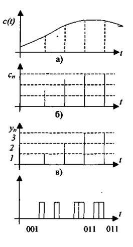
The conversion of a continuous primary analog signal into a digital code is called pulse code modulation(PCM). The main operations in PCM are the operations of time sampling, quantization (sampling by the level of a time-discrete signal) and coding.
Time sampling of an analog signal called a transformation in which the representing parameter of an analog signal is given by a set of its values at discrete times, or, in other words, in which from a continuous analog signal c(t)(Fig. 1.6, a) get sample values With"(Fig. 1.6, b). The values of the representing signal parameter obtained as a result of the time sampling operation are called samples.
The most widely used digital transmission systems, which use a uniform sampling of the analog signal (samples of this signal are made at regular intervals). With uniform discretization, the following concepts are used: sampling interval At(time interval between two adjacent samples of a discrete signal) and sampling frequency Fd(the reciprocal of the sampling interval). The value of the discretization interval is chosen in accordance with the Kotelnikov theorem.
According to the Kotelnikov theorem, an analog signal with a limited spectrum and an infinite observation interval can be reconstructed without errors from a discrete signal obtained by sampling the original analog signal if the sampling frequency is twice as high maximum frequency analog signal spectrum:
Kotelnikov's theorem
Kotelnikov's theorem (in the English literature - the Nyquist-Shannon theorem) states that if an analog signal x(t) has a limited spectrum, then it can be restored uniquely and without loss from its discrete samples taken with a frequency of more than twice the maximum frequency of the spectrum Fmax .